Creating a simple but funky to do list in Excel using data validation and Conditional Formatting

First of all, whilst I know there are a variety of apps out there can manage your to do lists (trello, todoist are some I continue to use) what I wanted here was a simple To Do list with some funky formatting that would allow me to standardise my list at work + share with colleagues and highlight certain aspects of the list…

I didn’t want to use a standard list because I wanted some visual alerts to progress on some of the lines and felt this was the best way.

Here’s what the finished spreadsheet looks like

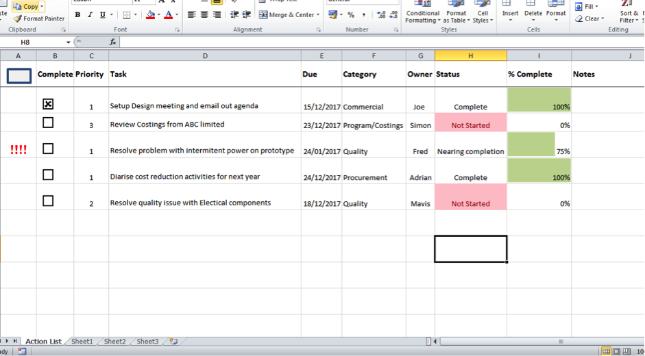
This to do spreadsheet works from 2 main sheets.

1/ “Action List” – this sheet contains the to do list

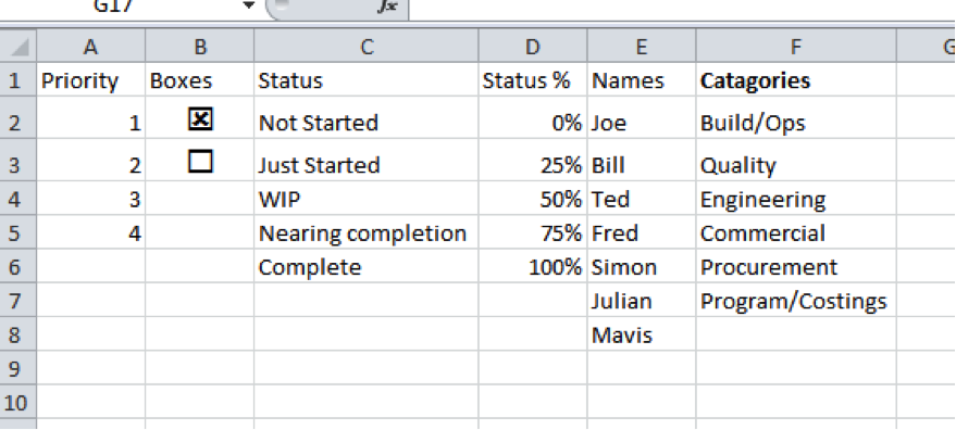
2/ “Sheet 1” – this sheet contains items I use for data validation or vlookups

How I build it

1/ In my “Action list” sheet I added my headers

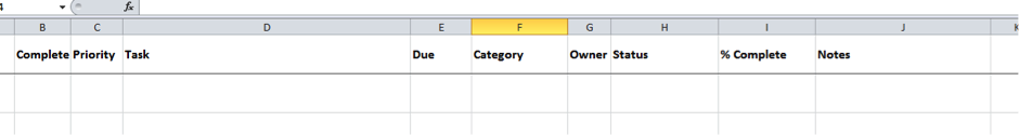
Note I left cell A1 empty so I could put in a “add a line button” which I’ll link to a Macro later.

2/ In Sheet 1 I added some columns to use with Data validation in my main to-do list. (note Column B uses the Windings font to show the boxes (the boxes use ý and ¨characters.

3/ Formatting rules on Action list tab

Let’s go through each column in detail.

Column A – my alert column – this basically uses a formulae to check if we’re passed the due date and if it is put some bright red exclamation marks in the cell. The formulae I used for this was…

=IF(B2=””,” “,IF(B2=Sheet1!$B$2,” “,IF(E2<TODAY(),”!!!!”,” “)))

Which in English means…

If B2 is empty – then nothing, if it’s got a checked box in it (note it’s called from my sheet 1 validation set) then no alert required as task is closed, if it’s open then go check the due date if it’s in arrears then put “!!!!” in it. I then used formatting to make them large and red.

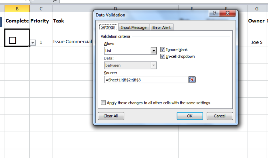
Column B – checkbox.

This uses data validation to pull through the check box from sheet 1

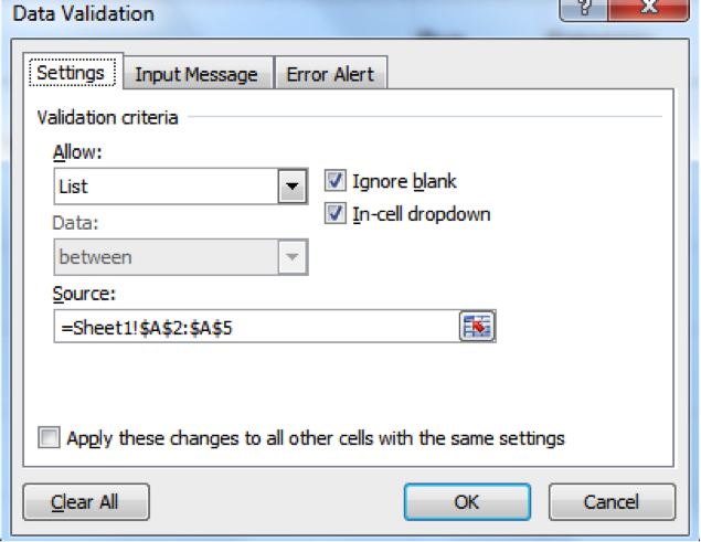
Column C

This uses data validation to pull through the priority

Column D – the task.

This is just a normal cell with “wrap text” feature enabled

Column E – Due

This is just a normal cell where I enter (in date format) the due date of the task

Column F – Category

This uses data validation to pull through the category from Sheet 1

Column G Owner

This uses data validation to pull through the task owner from Sheet 1

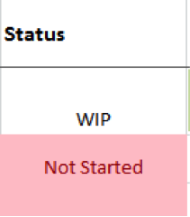
Column H Status

This uses data validation to pull through the task status from Sheet 1. I then use some Conditional formatting so that when the status is not started the cell is highlighted red with pink text (see pic below).

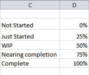
Column I % Complete

I use a Vlookup to return the value next to the status column on Sheet 1 – the formulae used is

=VLOOKUP(H2,Sheet1!$C$2:$D$6,2,FALSE)

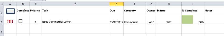
For example you can see the WIP (Work in progress) status has a % complete of 50% associated with it.

The reason I used standard % ‘s is that I wanted for other members of my project to use the sheet and I wanted a standard way of assessing progress – Yes, I know it’s not 100% accurate but it does give me a rule of thumb that I can use with the team-members.

With the Vlookup I used Conditional Formatting to put a data bar in the cell indicating progress – the settings are

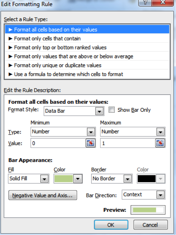
I really like this feature and it gives a good visual indication when you’re reviewing the list.

Column J – Notes – this is just a free text cell for adding any comments/notes about the task.

The add a line button.

In A1 – I added a square symbol – as below.

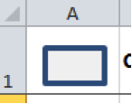
I then created a macro that basically copied the 2^nd row (the first with to’do’s in) then put it at the bottom of the table as a new line – the macro delete’s contents in the new line leaving it ready to have new data entered.

My Macro is:

Sub New_line()

‘ New_line Macro

Rows(“2:2”).Select

Selection.Copy

Range(“B1”).Select

Selection.End(xlDown).Select

ActiveCell.Offset(1, 0).Select

ActiveCell.Offset(0, -1).Select

ActiveSheet.Paste

ActiveCell.Offset(0, 3).Select

Selection.ClearContents